# Dr. M. Baron, Statistical Machine Learning class, STAT-427/627

# Regression with Dummy Variables and Interactions

> load("Auto.rda")

> attach(Auto)

> country = as.factor(origin)

> plot(weight,mpg)

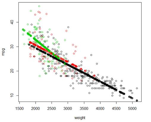
> plot(weight,mpg,col=country)

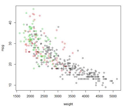
# Country appears to be an important variable that is not numerical.

> reg = lm(mpg ~ country)

> summary(reg)

Call:

lm(formula = mpg ~ country)

Residuals:

Min 1Q Median 3Q Max

-12.451 -5.034 -1.034 3.649 18.966

Coefficients:

Estimate Std. Error t value Pr(>|t|)

(Intercept) 20.0335 0.4086 49.025 <2e-16 ***

country2 7.5695 0.8767 8.634 <2e-16 ***

country3 10.4172 0.8276 12.588 <2e-16 ***

---

Signif. codes: 0 ‘***’ 0.001 ‘**’ 0.01 ‘*’ 0.05 ‘.’ 0.1 ‘ ’ 1

Residual standard error: 6.396 on 389 degrees of freedom

Multiple R-squared: 0.3318, Adjusted R-squared: 0.3284

F-statistic: 96.6 on 2 and 389 DF, p-value: < 2.2e-16

# R created dummy variables country2 and contry3

# Including INTERACTIONS

> reg = lm(mpg ~ weight*country)

# This is a short way to include weight, country, and all interactions

> summary(reg)

Call:

lm(formula = mpg ~ weight * country)

Residuals:

Min 1Q Median 3Q Max

-13.4928 -2.7715 -0.3895 2.2397 15.5163

Coefficients:

Estimate Std. Error t value Pr(>|t|)

(Intercept) 4.315e+01 1.186e+00 36.378 < 2e-16 ***

weight -6.854e-03 3.423e-04 -20.020 < 2e-16 ***

country2 1.125e+00 2.878e+00 0.391 0.69616

country3 1.111e+01 3.574e+00 3.109 0.00202 **

weight:country2 3.575e-06 1.111e-03 0.003 0.99743

weight:country3 -3.865e-03 1.541e-03 -2.508 0.01255 *

---

Signif. codes: 0 ‘***’ 0.001 ‘**’ 0.01 ‘*’ 0.05 ‘.’ 0.1 ‘ ’ 1

> reg = lm(mpg ~ weight*country)

> Yhat = fitted.values(reg) # Save Y-hat, the miles per gallon predicted by our new model

> points(weight,Yhat,col=country,lwd=3)

# Adding 3 fitted regression lines to the plot, one for each country! Col = color, lwd = line width